Calibrating species_radii

species_radii is the element-wise dictionary that controls how the free-volume Monte Carlo estimator decides whether a sampled point is occupied. Because \(V_{\mathrm{free}}\) enters the GCMC insertion and deletion acceptance terms directly (see Free volume and species_radii), the quality of these radii is a sensitive input – not a tuning knob to leave at default values.

The exclusion radius for a host species should reflect the shortest adsorbate-host distance that survives a local relaxation with the calculator used in production (the thesis behind this library denotes it \(r_{\mathrm{relax}}\)). Every value of species_radii is tied to the specific calculator and relaxation settings used during production; re-calibrate if either changes.

Free-volume estimate (recap)

For completeness, the estimator used by every cell object in mcpy is:

\[\begin{split}I_k = \begin{cases} 1, & \exists\, a\ \text{such that}\ \|\mathbf{x}_k-\mathbf{r}_a\|^2 \le r_{\mathrm{species}(a)}^2,\\ 0, & \text{otherwise,} \end{cases} \qquad V_{\mathrm{free}} = V_{\mathrm{cell}}\,\bigl(1 - \tfrac{1}{N_{\mathrm{MC}}}\textstyle\sum_k I_k\bigr).\end{split}\]

See Free volume and species_radii for the role of \(V_{\mathrm{free}}\) in the GCMC acceptance terms.

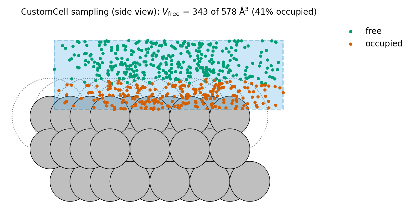
The estimator at work in a CustomCell over an Ag(111) slab, sampled by the cell itself (docs/make_figures.py). Each point drawn by cell.get_random_point() is classified against the exclusion disks of radius \(r_{\mathrm{Ag}}\) (dotted circles); the free fraction sets the \(V_{\mathrm{free}}\) that cell.get_volume() returns.

Measure the radius from relaxed insertions

Drop a trial adsorbate at random positions above the surface, relax each trial with your production calculator, and record the nearest adsorbate-host distance that survives:

import numpy as np
from ase.build import fcc111
from ase.constraints import FixAtoms
from ase.optimize import LBFGS

rng = np.random.default_rng(11)
slab0 = fcc111('Ag', a=4.085, size=(3, 3, 3), vacuum=8.0, periodic=True)
z_top = slab0.positions[:, 2].max()

distances = []
for _ in range(150):
    slab = slab0.copy()
    slab.set_constraint(FixAtoms(indices=[a.index for a in slab if a.tag == 3]))
    slab.append('O')
    slab.positions[-1] = [rng.uniform(0, slab.cell[0, 0]),
                          rng.uniform(0, slab.cell[1, 1]),
                          z_top + rng.uniform(1.0, 3.5)]
    slab.calc = calculator          # your production calculator
    LBFGS(slab, logfile=None).run(fmax=0.1, steps=50)
    d = slab.get_distances(len(slab) - 1, range(len(slab) - 1), mic=True)
    distances.append(d.min())

r_relax = np.percentile(distances, 5)   # edge of the first peak

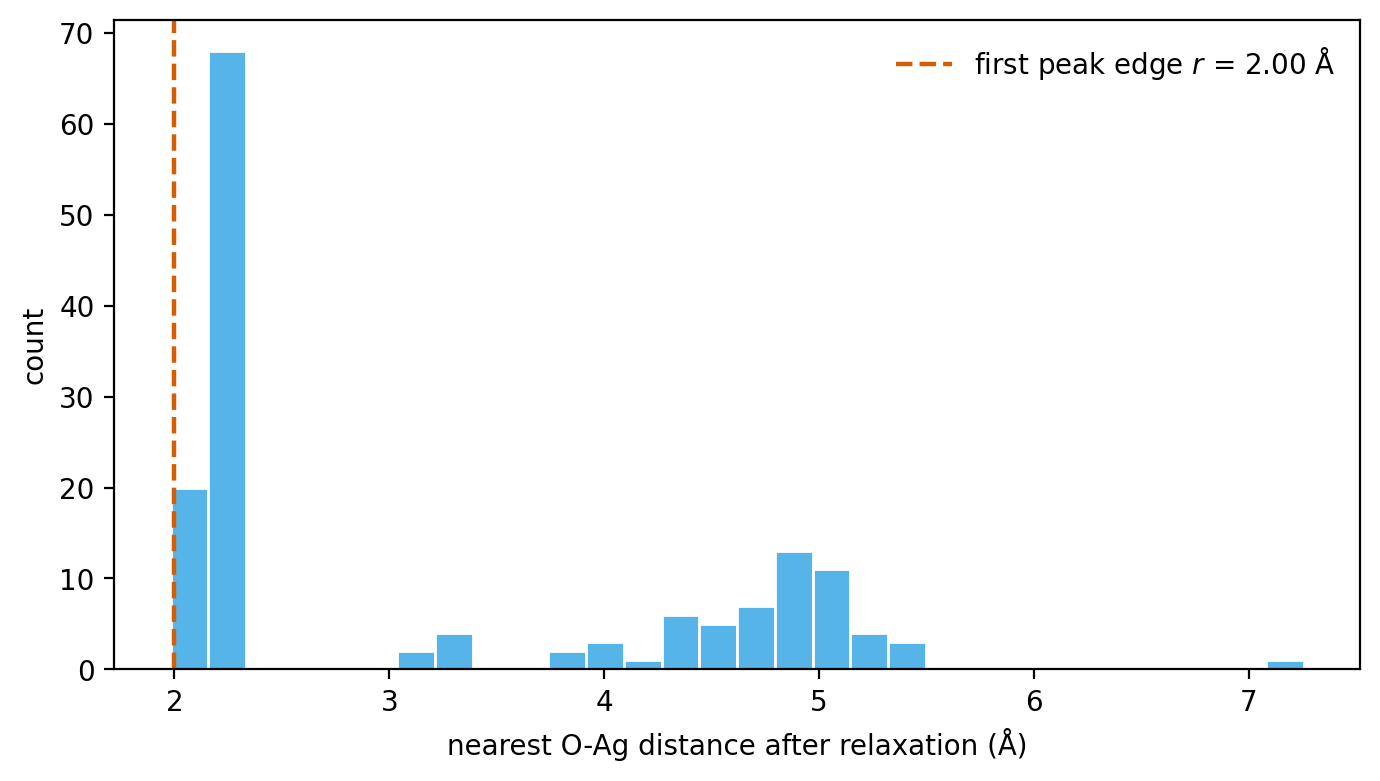
The histogram this loop produces (O on Ag(111); EMT stands in for the production calculator, generated by docs/make_figures.py). The sharp first peak collects the chemisorbed outcomes; its lower edge is \(r_{\mathrm{relax}}\).

The far cluster of large distances comes from trials that relaxed away without binding – ignore it and read off the lower edge of the first peak. scripts/compute_radii.py packages this loop for FCC(111) hosts with a MACE model.

Use the value in a simulation

Put the measured pair distance on the host species and zero on the adsorbate (or split it equally between the two – either convention works if used consistently):

cell = CustomCell(
    atoms,
    custom_height=5.0,
    bottom_z=atoms.positions[:, 2].max() + 0.5,
    species_radii={'Ag': r_relax, 'O': 0.0},
)

Validate with a short pilot run before production: the insertion acceptance ratio and the reported \(V_{\mathrm{free}}\) should both be stable and non-degenerate.