From a clean slab to an oxidation phase diagram

This tutorial builds a surface oxidation phase diagram. Starting from a clean Ag(111) slab, you will run grand-canonical Monte Carlo (GCMC) at a series of oxygen chemical potentials and turn the results into a figure that shows which oxide coverages are stable under which conditions. Every intermediate output is inspected along the way, so you can tell a healthy run from a broken one before committing real compute.

GCMC samples the compositions the reservoir conditions favour. You fix the temperature and the oxygen chemical potential, and the simulation inserts and deletes oxygen atoms until the surface reaches the coverage those conditions dictate. That equilibrium coverage, swept across chemical potentials, is the phase diagram.

1. Installing mcpy and checking the setup

mcpy installs from the repository. The mcpy name on PyPI belongs to an unrelated macro library, so clone and install from source (details in Installation).

The mace extra installs the MLIP backend. This tutorial evaluates energies with a MACE foundation model, and the extra pulls in mace-torch together with the packages the bundled examples use.

An import check confirms the install.

git clone https://github.com/farrisric/mcpy.git
cd mcpy
pip install -e .[mace]
python -c "import mcpy; print('mcpy', mcpy.__version__)"

2. Building the slab and marking where oxygen can go

Build the substrate

The starting configuration is a plain ASE Atoms object. Anything you can build with ASE can seed a run, and here fcc111 gives a 4x4x3 Ag slab with 8 Å of vacuum.

FixAtoms anchors the bottom layer. Trial moves are followed by a short relaxation, and without the constraint the whole slab would drift with every accepted move instead of representing a semi-infinite crystal.

Mark the insertion window

The CustomCell defines the insertion window. It spans the full width of the box but only a 5 Å slice starting above the top Ag layer, so every proposed oxygen lands near the surface instead of somewhere in the vacuum.

species_radii feeds the free-volume estimate. The cell measures how much of its window is not already occupied by atoms, counting a point as occupied when it falls within the given radius of an atom of that element, and that free volume enters the GCMC acceptance rule directly.

These radii deserve calibration before production runs. The values below are sane for O on Ag, and Calibrating species_radii shows how to derive them for your own potential and system.

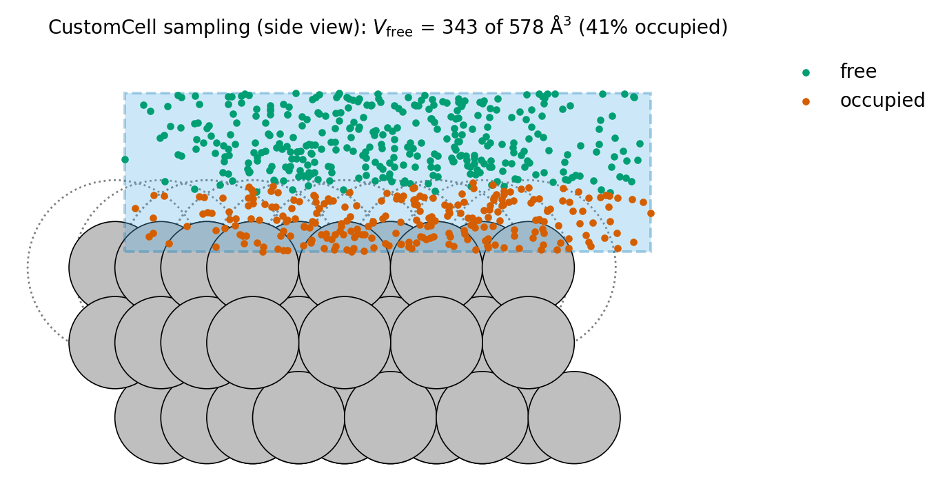
The CustomCell built above, sampled by its own machinery (docs/make_figures.py): the dots are draws from cell.get_random_point(), classified by the cell’s estimator, and the \(V_{\mathrm{free}}\) in the title is what cell.get_volume() reports and the acceptance rule uses.

from ase.build import fcc111
from ase.constraints import FixAtoms

from mcpy.cell import CustomCell

atoms = fcc111('Ag', a=4.085, size=(4, 4, 3), vacuum=8.0, periodic=True)
bottom = [a.index for a in atoms if a.tag == 3]
atoms.set_constraint(FixAtoms(indices=bottom))

cell = CustomCell(
    atoms,
    custom_height=5.0,
    bottom_z=atoms.positions[:, 2].max() + 0.5,
    species_radii={'Ag': 2.75, 'O': 0.0},
    mc_sample_points=100_000,
)

3. Choosing the trial moves

Composition changes need an insertion move and a deletion move. InsertionMove places a new O atom at a random point in the cell, rejecting draws that land within min_insert of an existing atom, and DeletionMove removes a random O atom from inside the cell. Together they let the oxygen count fluctuate, which is the defining feature of the grand-canonical ensemble.

MoveSelector draws one move per step. The weights are relative frequencies, so [1, 1] attempts insertions and deletions equally often, and the selector reports a separate acceptance ratio for each move in the log.

Explicit seeds make runs reproducible. Each move owns its random-number generator, and deriving both seeds from one SeedSequence means a single integer reproduces the entire run.

import numpy as np

from mcpy.moves import InsertionMove, DeletionMove
from mcpy.moves.move_selector import MoveSelector

ss = np.random.SeedSequence(42)
s1, s2 = (int(x) for x in ss.generate_state(2, dtype=np.uint32))

moves = MoveSelector(
    [1, 1],
    [InsertionMove(cell, species=['O'], min_insert=0.5, seed=s1),
     DeletionMove(cell, species=['O'], seed=s2)],
)

4. Wiring a calculator that relaxes each trial

MACE_F_Calculator relaxes each trial structure. It wraps a MACE model in a short LBFGS geometry optimization, and the energy handed to the acceptance rule is the relaxed one.

Raw insertions land far from real bonding sites. A random point in the free volume typically sits a fraction of an angstrom off the nearest hollow site, and evaluated as placed it carries a repulsive energy that would reject nearly every insertion. Relaxing first lets acceptance reflect the chemistry of the nearby minimum instead of the luck of the draw, which is what makes GCMC workable on a dense metal surface (see Calculators for the calculator options).

steps and fmax cap the relaxation budget. Forty optimizer steps to a loose 0.1 eV/Å tolerance is enough to absorb the placement noise, and a Monte Carlo run spends its budget better on more trials than on converging each one to machine precision.

from mcpy.calculators import MACE_F_Calculator

calculator = MACE_F_Calculator(
    model_paths='mace_mp_medium.model',   # your local MACE checkpoint
    steps=40,
    fmax=0.1,
    device='cuda',
)

5. Running GCMC at one chemical potential

Reference the chemical potential

The oxygen chemical potential references the O₂ molecule. The reservoir in an oxidation experiment is O₂ gas, so the natural zero for one adsorbed O atom is half the energy of an O₂ molecule computed with the same calculator.

\(\Delta\mu\) expresses the environmental conditions. Values below zero correspond to oxygen-poor conditions such as high temperature or low pressure, and values near zero to oxygen-rich ones. Here a single condition at \(\Delta\mu = -0.3\) eV serves as the test run before the sweep.

Assemble and run

GrandCanonicalEnsemble ties every ingredient together. It draws a move from the selector each step, evaluates the relaxed trial energy, applies the grand-canonical acceptance rule at the given mu and temperature, and commits or rolls back the configuration.

The write intervals control the two output files. Every accepted configuration goes to the trajectory, while the log gets one line every ten steps to stay readable. Expect the first step to be slower than the rest, since the model loads and the cell samples its free volume once up front.

from ase.build import molecule

from mcpy.ensembles.grand_canonical_ensemble import GrandCanonicalEnsemble

o2 = molecule('O2', cell=[12.0] * 3)
e_o2 = calculator.get_potential_energy(o2)

gcmc = GrandCanonicalEnsemble(
    atoms=atoms,
    cells=[cell],
    calculator=calculator,
    mu={'O': e_o2 / 2 - 0.3},     # half the O2 energy plus Delta mu = -0.3 eV
    units_type='metal',
    species=['O'],
    temperature=500.0,
    move_selector=moves,
    outfile='gcmc.out',
    traj_file='gcmc.xyz',
    outfile_write_interval=10,
    trajectory_write_interval=1,
)
gcmc.run(steps=1000)

Read the outputs

The log tracks particle count, energy, and acceptance ratios. Each line carries the step index, the current atom count, the current energy, and the acceptance ratio of every move since the previous line, in the move order spelled out in the header.

Step       N_atoms    Energy (eV)     Acceptance Ratios (Ins, Del)
-----------------------------------------------------------------
0          48         -157.210000     N/A, N/A
10         51         -160.830000     40.0%, 0.0%
...
1000       58         -168.120000     25.5%, 12.0%

The trajectory opens directly in ASE. Frames are extended XYZ with the energy and lattice on the comment line, so ase.io.read recovers everything the analysis below needs.

Convergence shows as a plateau in the oxygen count. Plot the count against the frame index, and treat the run as equilibrated only after the curve levels off and fluctuates around a steady value.

Unbalanced acceptance ratios signal an unconverged run. While coverage is still climbing, insertions far outpace deletions, and in the steady state the two ratios settle to comparable values. A persistent imbalance after the count has flattened points at mis-calibrated exclusion radii instead.

from ase.io import read

traj = read('gcmc.xyz', index=':')
n_oxygen = [sum(a.symbol == 'O' for a in frame) for frame in traj]
# plot n_oxygen vs frame index: it should plateau in the second half

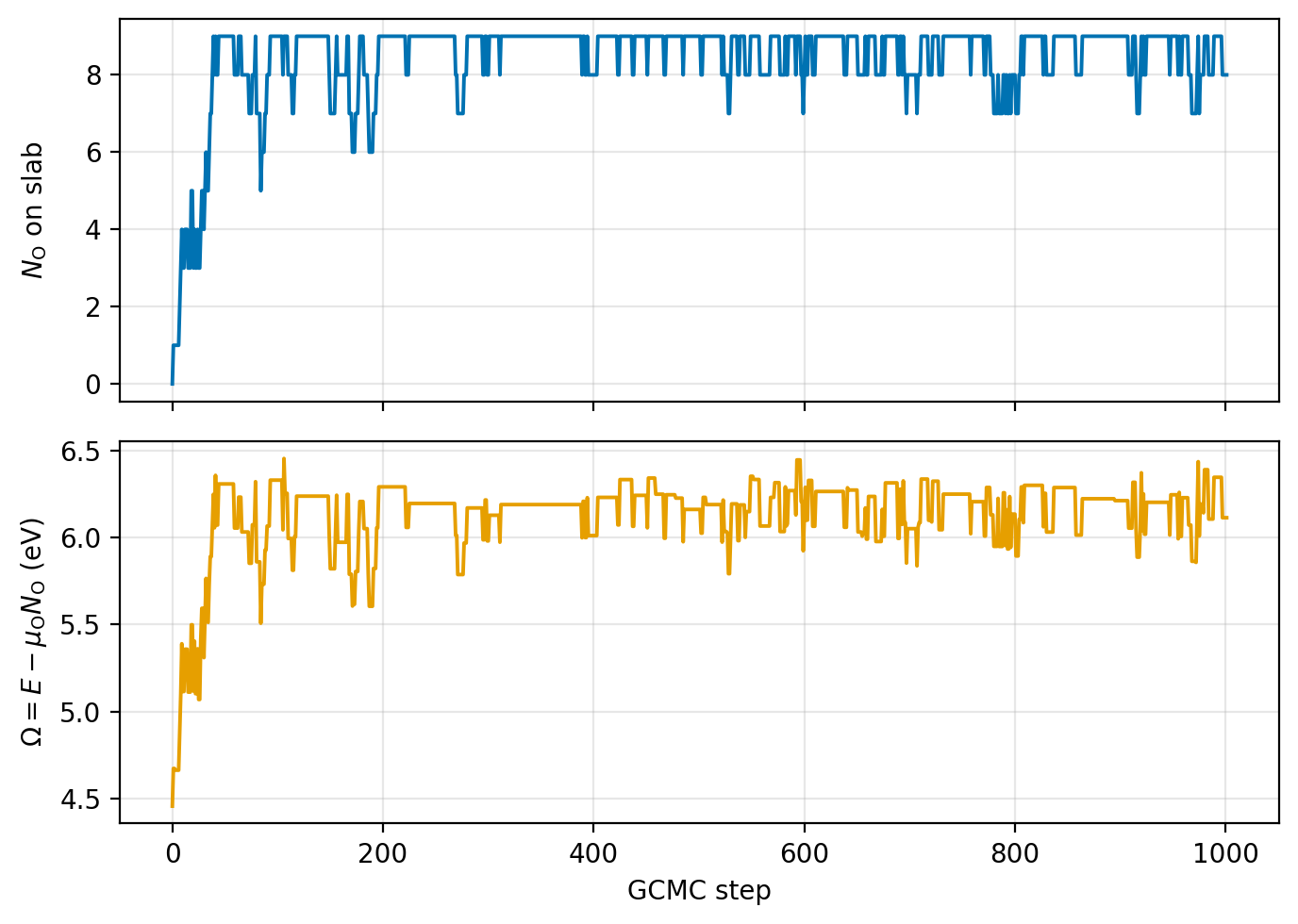
What a healthy run looks like: a 1000-step EMT demo of this setup (generated by docs/make_figures.py). The oxygen count climbs from the clean slab and fluctuates around one monolayer, and the grand potential \(\Omega = E - \mu_{\mathrm{O}} N_{\mathrm{O}}\), the quantity GCMC drives downhill, decreases and then levels off. EMT’s toy O-Ag energetics need two demo-specific settings, documented in the script: \(\mu_{\mathrm{O}} = -0.2\) eV on EMT’s energy scale, and a one-monolayer max_atoms cap on the insertion move.

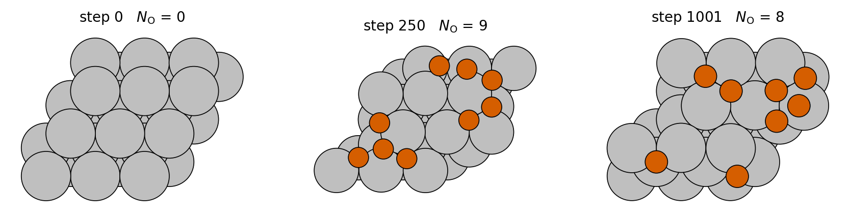
Trajectory snapshots from the same run (top view, O in orange): the clean starting slab, the climb, and the equilibrated monolayer.

6. Sweeping the chemical potential

One run samples one environmental condition. The phase diagram needs the equilibrium answer at several chemical potentials, and each one is an independent GCMC run that can execute in sequence or in parallel.

A function parameterised on \(\Delta\mu\) drives the sweep. The body repeats sections 2 through 5 unchanged, so only the chemical potential and the output paths vary between conditions.

Each condition writes into its own directory. Condition-tagged paths keep the sweep restartable and make the collection step below a one-liner.

The early frames belong to equilibration. Every run starts from the same clean slab, so the first stretch of each trajectory records the climb toward equilibrium rather than samples of it, and the analysis will drop those frames.

from pathlib import Path

def run_gcmc(delta_mu, steps=1000, seed=42):
    outdir = Path(f'sweep/dmu_{delta_mu:+.2f}')
    outdir.mkdir(parents=True, exist_ok=True)
    # rebuild atoms, cell, moves, and calculator exactly as in
    # sections 2-4, seeded per condition
    ...
    gcmc = GrandCanonicalEnsemble(
        ...,
        mu={'O': e_o2 / 2 + delta_mu},
        outfile=str(outdir / 'gcmc.out'),
        traj_file=str(outdir / 'gcmc.xyz'),
    )
    gcmc.run(steps=steps)

for delta_mu in (-0.8, -0.6, -0.4, -0.2, 0.0):
    run_gcmc(delta_mu)

7. Assembling the phase diagram

Collect the frames

The sweep trajectories are the input. mcpy.utils.phase_diagram.plot_phase_diagram() accepts a list of trajectories and flattens them, so passing one production slice per condition is enough.

The clean slab serves as the reference. Formation energies are measured against the lowest-energy oxygen-free frame in the input, and since the production slices start after equilibration, frame 0 of one run is kept to guarantee a clean reference exists.

Draw the diagram

plot_phase_diagram computes the surface formation energy per frame. For every frame it evaluates the formation energy as a function of \(\Delta\mu\) from the frame’s energy and oxygen count, normalised by the surface area.

The lower envelope marks the stable phases. At each \(\Delta\mu\) the frame with the lowest formation energy wins, and the winning stretches partition the axis into the stable coverages.

The transitions array locates the phase boundaries. Each entry is the \(\Delta\mu\) where the envelope switches from one structure to the next, and a twin axis converts the range into O₂ pressures at the given temperature.

Thumbnails show one structure per stable phase. The figure renders the winning configuration of each stretch above the envelope, so the diagram reads as structures, not curve indices. Building phase diagrams from GCMC output covers every knob, including nanoparticle normalisation and molecular adsorbates.

from ase.io import read

from mcpy.utils.phase_diagram import plot_phase_diagram

# The lowest-energy O-free frame is the reference, so keep frame 0
# (the clean slab) even though the equilibration frames are dropped.
clean = read('sweep/dmu_-0.80/gcmc.xyz', index='0')

frames = [clean] + [
    read(f'sweep/dmu_{dmu:+.2f}/gcmc.xyz', index='500:')   # drop equilibration
    for dmu in (-0.8, -0.6, -0.4, -0.2, 0.0)
]

results = plot_phase_diagram(
    frames,
    adsorbate='O',
    metal_symbols=('Ag',),
    mu_ref=e_o2 / 2,
    kind='surface',
    T=500.0,
    dmu_range=(-1.0, 0.0),
    outfile='phase_diagram.png',
)
print(results['transitions'])   # Delta mu values of the phase boundaries

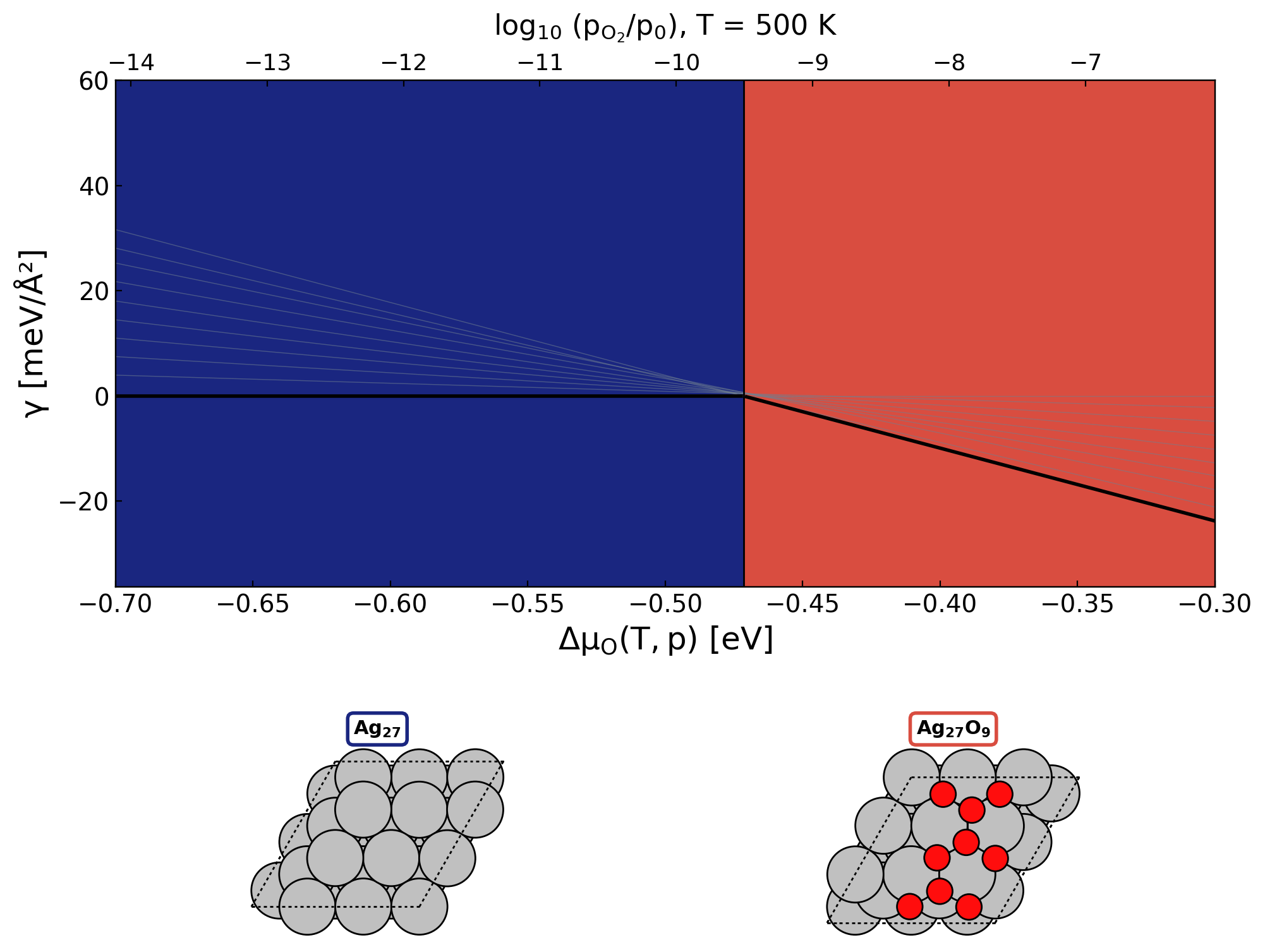
The diagram this exact call produces on the EMT demo sweep (docs/make_figures.py). Grey lines are individual frames, the thick line is the stable envelope, and the shading marks the stable phases, labelled by their structure thumbnails: the clean slab below \(\Delta\mu_{\mathrm{O}} \approx -0.47\) eV and the one-monolayer phase above it. The top axis converts \(\Delta\mu_{\mathrm{O}}\) into O₂ pressure at 500 K. For a production-quality MACE example see Building phase diagrams from GCMC output.

8. Where to go next

Production runs need calibrated exclusion radii. Calibrating species_radii derives them from relaxed insertion trials with your own potential.

Molecular adsorbates exchange whole molecules with the reservoir. Simulating molecular adsorbates covers rigid insertion, deletion, and displacement of species such as CO and O₂.

Replica exchange runs every condition in parallel. Ensembles describes the MPI and single-GPU batched variants, either of which can replace the sequential loop of section 6.

Other cells fit nanoparticles and supported particles. Cells maps each geometry to its cell type, from periodic boxes to spheres and domes.

The notebooks repeat these workflows with executed output. The notebooks page lists them, from GCMC basics to the CO/CuPd replica-exchange study, with every cell already run.