Building phase diagrams from GCMC output

mcpy.utils.phase_diagram.plot_phase_diagram() turns the trajectories of a chemical-potential sweep into a phase diagram: it computes the formation energy of every frame, takes the lower envelope over a \(\Delta\mu\) grid, and renders the figure with a structure thumbnail per stable phase.

Build the diagram from a sweep

Collect one production slice per condition, keep one adsorbate-free frame as the clean reference (the function raises an error without one), and call the function:

from ase.io import read

from mcpy.utils.phase_diagram import plot_phase_diagram

# keep frame 0 (the clean starting slab) as the reference
clean = read('sweep/dmu_-0.80/gcmc.xyz', index='0')

frames = [clean] + [
    read(f'sweep/dmu_{dmu:+.2f}/gcmc.xyz', index='500:')   # drop equilibration
    for dmu in (-0.8, -0.6, -0.4, -0.2, 0.0)
]

results = plot_phase_diagram(
    frames,
    adsorbate='O',
    metal_symbols=('Ag',),
    mu_ref=e_o2 / 2,          # adsorbate reference on your calculator's scale
    kind='surface',           # or 'nano' for nanoparticles
    T=500.0,
    dmu_range=(-1.0, 0.0),
    outfile='phase_diagram.png',
)
print(results['transitions'])   # Delta mu values of the phase boundaries

frames takes a flat list of Atoms or a list of trajectories and flattens them; frames written by mcpy carry their energy on the comment line, so nothing is re-evaluated. The returned dict carries the grid (dmu_grid), the per-frame lines (free), the envelope (min_gamma), the winning frame indices (stable_idx, phase_order), and the boundary positions (transitions).

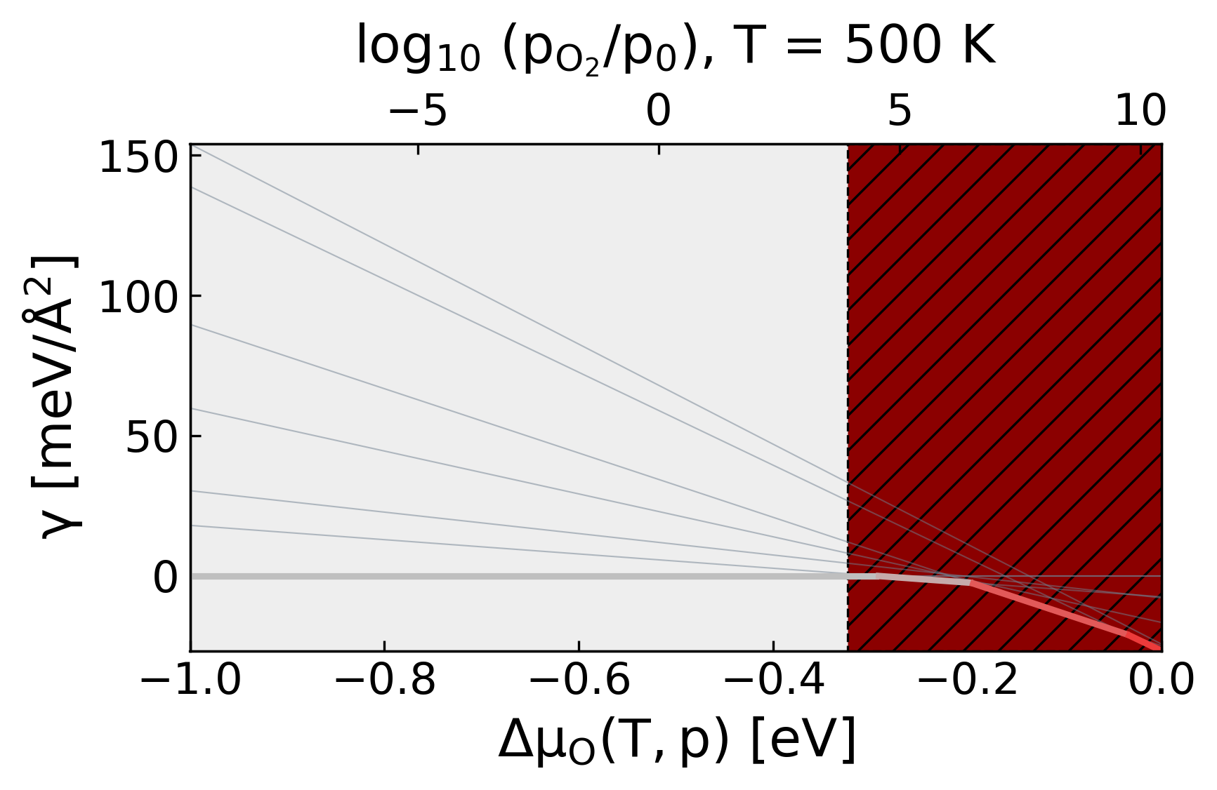
Surface phase diagram of O on Ag(111). — A surface diagram (O on Ag(111), MACE). Grey lines are individual frames, the thick line is the stable envelope, the shading marks the stable phases, and the top axis converts \(\Delta\mu_{\mathrm{O}}\) into O₂ pressure.

Key parameters

kind: 'surface' normalizes by the in-plane cell area (meV/Å²); 'nano' normalizes by the metal-atom count (meV/atom), which keeps particles of different sizes comparable. gamma_in_ev=True skips the normalisation.
mu_ref: The adsorbate reference on your calculator’s energy scale, for example half the O₂ energy. The twin pressure axis converts \(\Delta\mu\) at the given T.
n_bins / min_phase_width: Resolution of the \(\Delta\mu\) grid, and the width below which near-degenerate phases merge into their neighbours.
adsorbate_count_fn / adsorbate_label: A custom atoms -> int counter for adsorbates whose element also sits in an inert sublattice (for example O adsorbed on a particle supported by an oxide), and the species name used in axis labels when the counted symbol is a proxy.
atoms_per_reservoir_molecule: Reservoir stoichiometry for the pressure axis. The default 2 is the dissociative-diatomic convention (atomic O from an O₂ reservoir); pass 1 for molecular adsorbates such as CO, whose thumbnails then read as (CO)_n.

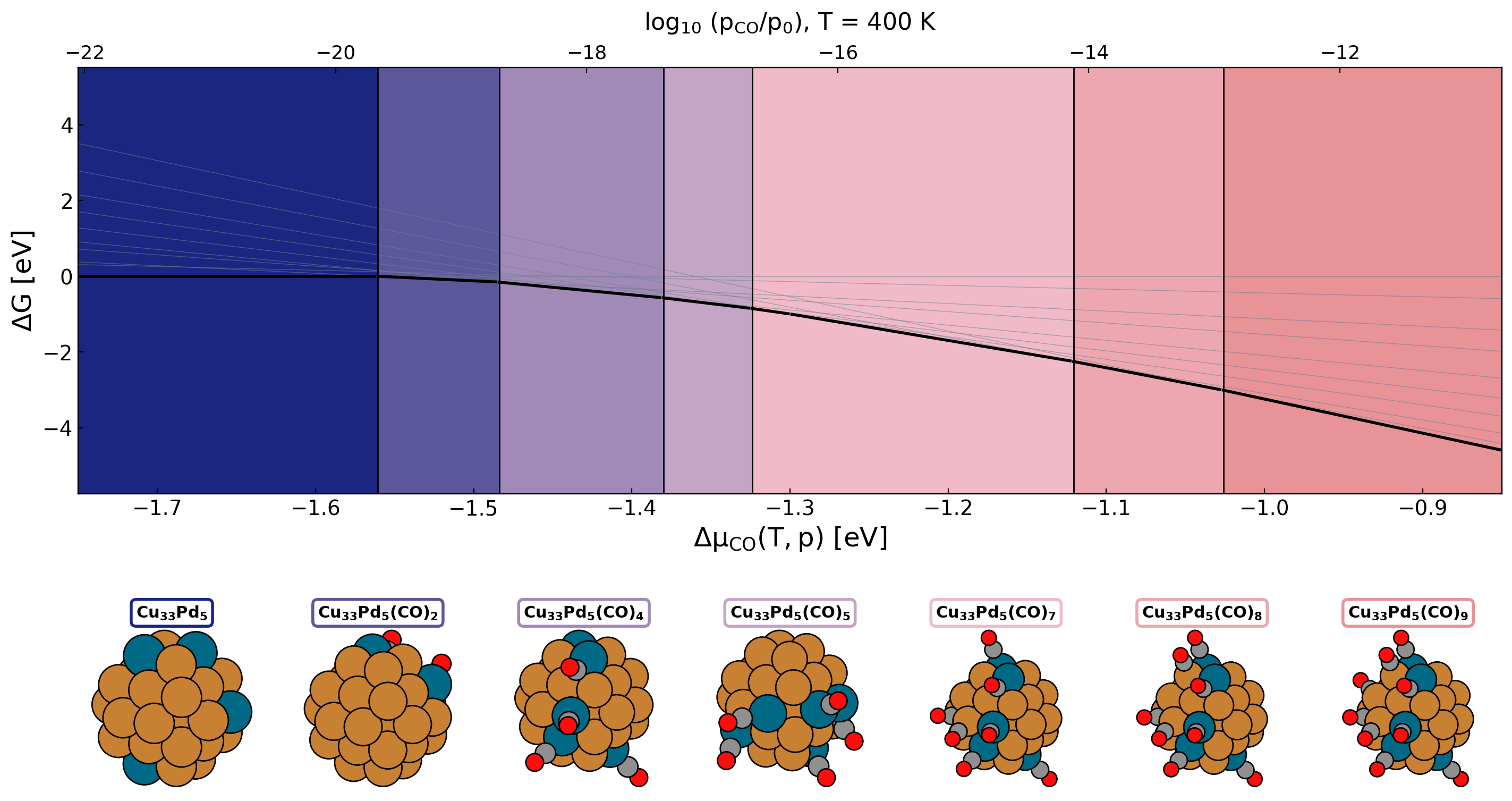
Phase diagram of CO on a CuPd nanoparticle with structure thumbnails. — A molecular nanoparticle diagram (CO on Cu₃₃Pd₅, `kind='nano'`, `atoms_per_reservoir_molecule=1`).

analyze_phase_diagram_results(trajectory_path, host_symbol, oxygen_symbol, idx_ref, ...): The older oxidation-specific entry point: reads one concatenated trajectory from disk and works against tabulated host and oxide reference energies. Prefer plot_phase_diagram for new work.

Worked examples

Section 7 of From a clean slab to an oxidation phase diagram builds the O/Ag(111) diagram from the tutorial sweep.
The phase-diagram notebook builds a diagram interactively with executed output (see Notebooks).
The CO/CuPd replica-exchange notebook ends in the molecular nanoparticle diagram above.