Phase diagram analysis from relaxed trajectories
This example shows how to analyze relaxed structures and construct a phase-diagram plot
using the utility function in mcpy.utils.phase_diagram.
The script evaluates the phase stability of each relaxed frame as a function of the oxygen chemical potential \(\Delta\mu_O\) and selects the lowest-energy structure across the sweep.
Example output
The figure below was produced by running a short MACE-MP sweep across
\(\Delta\mu_O \in \{-0.6, -0.3, 0.0, +0.3\}\,\mathrm{eV}\) on an
Ag(111) 3×3×3 slab at \(T = 500\,\mathrm{K}\) (248 GCMC frames total),
then feeding the merged trajectory into analyze_phase_diagram_results.
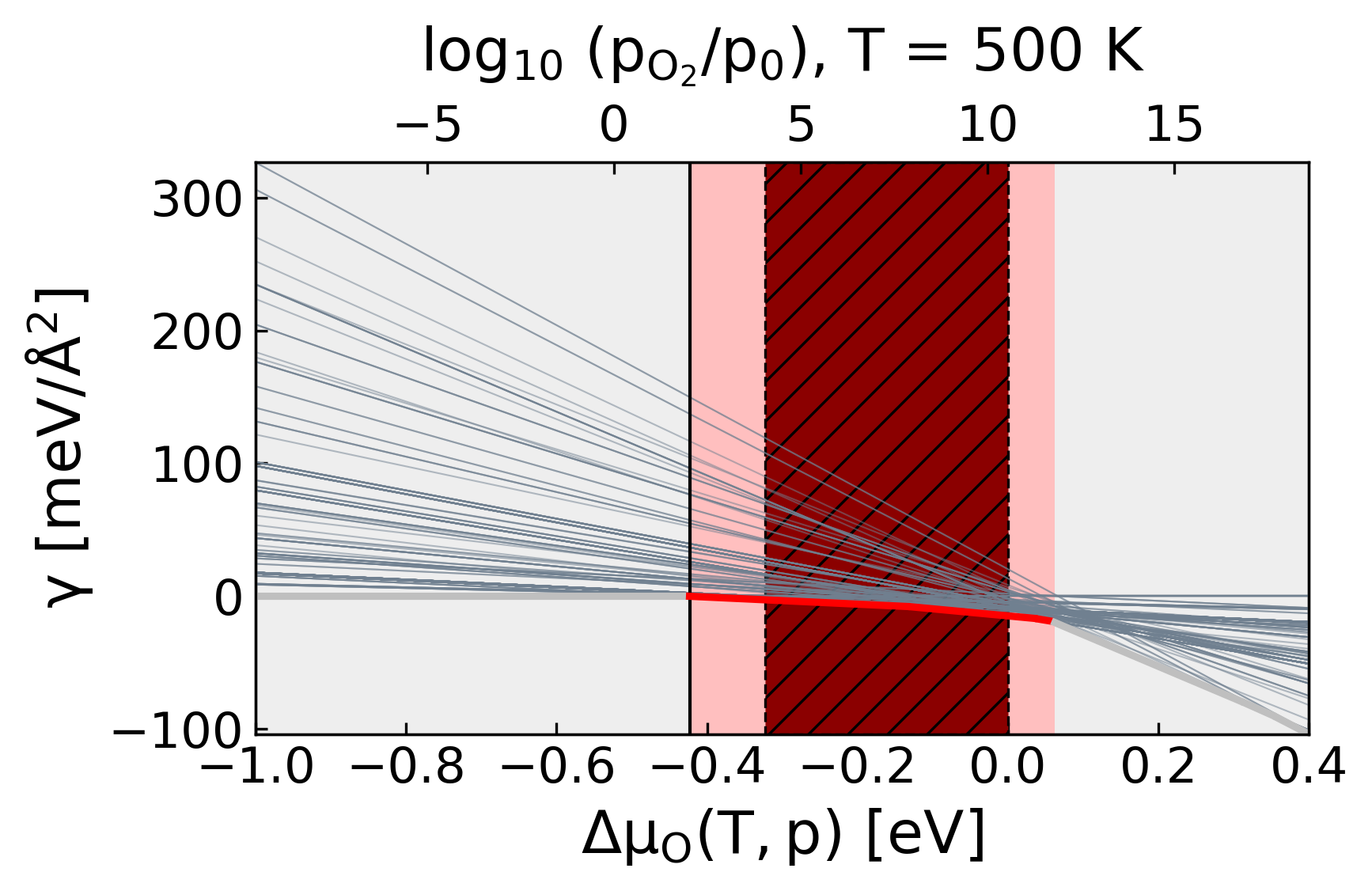
Surface Gibbs energy \(\gamma(\Delta\mu_O)\) for every relaxed configuration in the sweep (gray lines). The colored envelope marks the stable phase at each \(\Delta\mu_O\); vertical bands separate distinct stable phases. The hatched dark-red region indicates \(\Delta\mu_O > -\Delta H^f_{\mathrm{Ag}_2\mathrm{O}}\), where bulk Ag2O is more stable than any surface phase.
What to read off the plot:
Phase transitions appear as kinks in the lower envelope; the \(\Delta\mu_O\) values are returned in
transitions_delta_mu_o.Color intensity encodes the surface oxide ratio (O atoms divided by top-layer Ag atoms above
z_threshold).The leftmost band corresponds to the clean reference slab (
idx_ref); rightward bands carry increasing O coverage.
Thermodynamic model (from the thesis)
For an oxidized configuration at given oxygen chemical potential, the thesis uses the oxygen-dependent formation Gibbs energy. For surfaces, this is written in terms of the surface Gibbs energy \(\gamma\):
where \(E\) is the DFT energy of the relaxed configuration, \(n_{\mathrm{Ag}}\) and \(n_{\mathrm{O}}\) are atom counts, and \(A\) is the surface area.
The oxygen chemical potential \(\mu_{\mathrm{O}}(T,p)\) is expressed as
To correct DFT overbinding of O$_2$, the thesis replaces \(\tfrac{1}{2}E^{\mathrm{DFT}}_{\mathrm{O}_2}\) using the experimental formation enthalpy of the corresponding oxide:
In the code, this correction is embedded in e_o2 (see mcpy/utils/phase_diagram.py).
How utils/phase_diagram.py finds stable phases
The function computes \(\gamma(\Delta\mu_O)\) for each relaxed structure and selects the minimum at each chemical potential value. Concretely, it performs the following loop:
Load all frames from
relaxed_structures.xyz.Define a grid of oxygen chemical-potential offsets \(\Delta\mu_O\) (
delta_mu_oin the code).For each structure
confand each \(\Delta\mu_O\), compute the surface Gibbs energy density \(\gamma\) using the DFT energy, atom counts, the corrected oxygen reference energye_o2, and the surface area \(A\). In the implementation, this is done byfree_en(...)and then shifted so that the reference structure atidx_refdefines \(\gamma_{\mathrm{ref}}\).For each \(\Delta\mu_O\) bin, select the index of the stable phase as
argminof \(\gamma\) over all configurations.Detect transition points when the stable phase index changes between neighboring bins; these are returned as
transitions_delta_mu_o.
Importing the analysis helper
from mcpy.utils.phase_diagram import analyze_phase_diagram_results

result = analyze_phase_diagram_results(
    trajectory_path="relaxed_structures.xyz",
    idx_ref=2400,
    output_plot_path="lines_phases_mace.png",
    show_plot=False,
)

print("Transition points (delta mu_O):", result["transitions_delta_mu_o"])
print("Stable configuration indices:", result["stable_conf_idx"])
print("Saved plot:", result["plot_path"])
Inputs and outputs
Inputs:
trajectory_path: path to an ASE-readable trajectory (e.g.
.xyz) containing the relaxed structures you want to classify.idx_ref: reference frame index used to define
\\gamma_{\\mathrm{ref}}(a constant energy offset that shifts the whole phase diagram line).output_plot_path: where to save the generated phase-diagram plot.
show_plot: whether to display the plot interactively.
Outputs:
transitions_delta_mu_o: oxygen chemical-potential offsets where the stable phase changes.
stable_conf_idx: the index of the lowest-energy configuration at each
\\Delta\\mu_Obin.phase_oxide_ratios: a per-phase oxide ratio used for coloring.
plot_path: path to the saved figure.
What this function does
Loads all frames from relaxed_structures.xyz.
Computes free-energy lines as a function of \(\Delta\mu_O\).
Finds the lowest-energy structure at each \(\Delta\mu_O\).
Detects transition points between stable phases.
Highlights phase regions with background color bands and a color-changing stable-energy line.
Saves the resulting plot (lines_phases_mace.png by default).
Command-line usage
You can still run the same analysis script directly:
python -m mcpy.utils.phase_diagram relaxed_structures.xyz \
    --idx-ref 2400 --output lines_phases_mace.png
General adsorbate phase diagrams from multiple trajectories
analyze_phase_diagram_results above is tailored to oxygen-on-silver surfaces
(it embeds the oxide formation-enthalpy correction and a single input
trajectory). For a generic single-adsorbate system that was sampled across a
range of chemical potentials and split across many trajectory files, use
mcpy.utils.plot_phase_diagram() instead.
One call builds the diagram for one configuration (e.g. a single surface facet or a single nanoparticle size). You pass the in-memory frames belonging to that configuration; the function merges them, picks the lowest-energy adsorbate-free frame as the reference, and selects the stable phase at each \(\Delta\mu\). Both extended surfaces (normalized per surface area, meV/Ų) and nanoparticles (normalized per metal atom, meV/atom) are supported.
import glob
from ase.io import read
from mcpy.utils import plot_phase_diagram

# All trajectory files for ONE configuration (here a PdAg(111) surface,
# sweeping the H chemical potential across several runs/ranks).
files = sorted(glob.glob("results/regcmc_surface_111/PdAg_111_dmu_*_rank_*.xyz"))
frames = [read(f, ":") for f in files]   # list of trajectories, flattened internally

result = plot_phase_diagram(
    frames,
    adsorbate="H",
    metal_symbols=("Pd", "Ag"),
    mu_ref=-3.05,            # reference adsorbate chemical potential, e.g. 1/2 E(H2)
    kind="surface",          # "surface" -> meV/Ų; "nano" -> meV/atom
    T=300.0,
    dmu_range=(-1.0, 0.0),
    system_label="surface_111",
    outfile="figures/phase_surface_111.png",
)

print("Transitions (delta mu):", result["transitions"])
print("Stable phases (H counts):", [result["stoich"][i] for i in result["phase_order"]])
To process several configurations, call the function once per configuration with
the kwargs that differ between systems (the trajectory list, kind,
metal_symbols/adsorbate, system_label, outfile):
systems = {
    "surface_111": dict(glob="results/regcmc_surface_111/PdAg_111_dmu_*_rank_*.xyz",
                        kind="surface"),
    "nano_small":  dict(glob="results/regcmc_nano_small/PdAg_nano_small_dmu_*_rank_*.xyz",
                        kind="nano"),
}
for name, cfg in systems.items():
    frames = [read(f, ":") for f in sorted(glob.glob(cfg["glob"]))]
    plot_phase_diagram(frames, adsorbate="H", metal_symbols=("Pd", "Ag"),
                       mu_ref=-3.05, kind=cfg["kind"], system_label=name,
                       outfile=f"figures/phase_{name}.png")
Key parameters
frames: a flat list ofase.Atomsor a list of trajectories (each a list of frames); the latter is flattened automatically.adsorbate: symbol whose count defines the stoichiometry (e.g."H").metal_symbols: host species, used for per-atom normalization and the structure-thumbnail labels.mu_ref: reference chemical potential of the adsorbate [eV].kind:"surface"or"nano"(selects the normalization).min_phase_width: phases narrower than this \(\Delta\mu\) width are merged into a neighbor, suppressing spurious slivers.show_structures: render the per-phase structure thumbnails (defaultTrue; requiresase.visualize.plot). SetFalsefor the plot panel only.
Returns a dictionary with dmu_grid, free, stoich, stable_idx,
min_gamma, transitions, phase_order, phase_ratios, unit and
plot_path.